The AAA methodology for optimized implementation

3 The AAA methodology for optimized implementation

The AAA methodology is based on graphs in order to model the algorithm as well as the architecture. Therefore, a possible implementation of an algorithm onto an architecture may be specified as a graph transformation. The adequation amounts to choose among all the possible implementations (graphs transformations), the one which satisfies real-time and embedding constraints, corresponding to the optimized implementation. Finally, the code generation is an ultimate graph transformation leading to a distributed real-time executive for the multicomponents and to a structural hardware description, e.g. structural VHDL, for the specific integrated circuits. This graph oriented approach relies on a formal framework where it is possible to describe and verify all the steps from the specification to the real-time execution of the application. This allows to ensure a high level of dependability because there is actually no gap between these steps.

Moreover, if fault tolerance is specified at the level of the application by the user who describes the redundant computation and communication resources, then it is also possible to automatically add redundant operations and data dependences to the algorithm graph, which are taken into account during the implementation and the optimization, guaranteeing the behavior of the application if the specified hardware components fail. This issue will not be addressed here, but the interested reader may consult [8, 9].

3.1 Algorithm model

3.1.1 Control and data flow graphs

There are two main approaches for specifying an algorithm: the control flow and the data flow. In both cases the algorithm may be modeled by a directed graph [10]. It is the meaning given to the edges, which will differentiate both approaches. Briefly, we remind the reader that a graph (V,E) is a pair of sets, the set of vertices V and the set of edges E, each edge e = (v,w) being a pair of vertices, and then E ⊆ V × V. Directed means that the order of the vertices in the pair (v,w) is considered, whereas in non directed graphs it is not.

A “program flow chart” is a typical example of control flow graph, usually used before programming with an imperative language like C. Each vertex of such a graph represents an operation which consumes from, and produces data into variables during its execution, and each edge represents an execution precedence relation between the two operations. Actually, an edge is a sequence control which corresponds either to an unconditional (back or forth) or to a conditional branching. This latter is the basic mechanism when an operation or a subgraph of operations must be conditioned for example by the result of a test (“if …then …else …”). The notion of iteration or loop (“for i=1 to n do …”), related to unconditional back branching, corresponds to a temporal repetition (in opposition to spatial repetition used later on) of an operation, or of a subgraph of operations. A “state chart” is another commonly used control flow graph, where each vertex represents one of the possible states, and each edge represents a transition, from one state to another one, triggered by the arrival of an event. Each transition leads to execute an operation which consumes from and produces data into variables. In both cases the set of all edges defines a total order on the execution of all operations. There is no potential parallelism directly specified in this model, although it might be extracted from a data dependence analysis through the variables in which the operations read and write data. However, in the general case this analysis is very complicated and may conclude that no potential parallelism is available in this control flow graph. Moreover, there is no relationship between the order in which the operations must be executed, and the order in which these operations consume (read) from and produce (write) their data into the variables. Another way to specify potential parallelism consists in composing several control flow graphs which will communicate through shared variables. This approach is similar to CSP (Communicating Sequential Processes) [11].

In the basic data flow graph [12] each vertex represents an operation which consumes data before its execution and produces data after its execution, thus introducing a relationship between the order in which the operations must be executed and the order in which these operations consume and produce their data. The data produced by an operation and consumed by another one corresponds to a data transfer. Note that the notion of variable does not exist in this model; it is replaced by the notion of data transfer or “data flow”. This approach is also called “unique assignment” avoiding the problem related to shared variables. Each edge represents a data dependence inducing an execution precedence relation between two operations. An operation which does not need to transfer data to another operation is not connected by an edge to this operation. Consequently, the set of edges defines a partial order relation on the execution of all the operations [13, 14], defining in turn the potential parallelism of the data flow graph. The level of potential parallelism of a data flow graph depends on the lack of data dependences relatively to all the possible data dependences in the graph. There are two kinds of potential parallelism, data potential parallelism, usually called “data parallelism” when the operations without data dependences are the same (i.e. the same operation is applied to different data), and operation potential parallelism, usually called “task parallelism” when operations are different. Furthermore, because edges represents data transfers, hyper-edges (n-uples of vertices) are needed rather than edges (pairs of vertices) when it is necessary to specify that a data produced by an operation is consumed by more than one operation, corresponding to a data diffusion. This category of graph is called “hyper-graph”. Finally, a data flow graph is “acyclic” meaning that any path in the graph, formed by a succession of vertices and edges, must not have the same extremities which would produce a cycle. Cycles must be avoided because they introduce indeterministic behavior in the graph execution.

3.1.2 Factorized conditioned data dependence graph

The algorithm model [15, 16, 17] used in the AAA methodology allows to specify potential parallelism, to ensure coherence between the execution order of the operations and the way they consume and produce data, to avoid shared variables which are the source of numerous errors. This model is an extension of the basic data flow model in three directions. First we need to repeat infinitely and finitely a data flow graph pattern in order to take into account respectively the reactive aspect of the real-time systems and potential data parallelism. Second we need to specify “states” when data dependences are necessary between infinite repetitions. Third we must be able to condition the execution of several alternative data flow graphs according to the value transfered by a control dependence. Moreover, this model follows the synchronous language semantics [1], that is, physical time is not taken into account. Regarding one reaction of the system, that is, one data flow graph pattern of the infinite repetition, this means that each operation produces its output events instantaneously with the consumption of its inputs events which must be present altogether. Consequently it means that this data flow graph pattern is instantaneously executed. The successive executions of the data flow graph pattern introduces a notion of “logical instant”, using an additional precedence dependence (without data) between each repetition of the data flow graph pattern which ensures that a reaction will complete before another one begins. Each input or output of an operation carries an infinite sequence of events taking values which is called a “signal”. The union of all the signals define a “logical time”, such that physical time elapsing between events is not considered. Finally in order to limit the complexity of the graph, our model is factorized, that is, only the repeated data flow graph pattern is represented instead of all its repetitions (infinite or finite), leading to a factorized conditioned data dependence graph.

When an application is running, the reactive system (controller of equation 1) is infinitely repeated interacting with a physical environment through, let us say to simplify, one sensor and one actuator. In order to specify the maximum of potential parallelism, it is possible to “unroll” this infinite temporal repetition (iteration) in an infinite spatial repetition, assuming that it exists an infinity of sensors and actuators. This allows to model the algorithm corresponding to the controller as an infinitely repeated data flow graph pattern. However, in order to simplify its large specification, it is only necessary to describe one instance of this data flow graph repetition, and then it is said infinitely factorized. When an instance of the factorized data flow graph needs a data produced by an operation belonging to a previous instance corresponding to an inter-repetition data dependence, this induces a cycle which must be mandatory avoided (acyclic graph) by introducing a specific vertex called delay. It is equivalent to the well known z⁻ⁿ used in control and signal processing theory. The set of all the delays memorizes the algorithm state. Actually a delay is equivalent to two vertices containing a memory: one vertex without predecessor and one vertex without successor. The value contained in the memory of the latter vertex is copied in the other memory at the end of each reaction (data flow graph pattern execution). Moreover, another advantage of the data flow approach, is that the algorithm state is clearly localized in the delay vertices, whereas in the control flow approach it is spread out in all the variables. This issue is especially important when dealing with control and signal processing algorithms where state must be carefully mastered. It is also possible to repeat spatially an operation, or a subgraph of operations, N times (finitely), but represented as a single graph with a label indicating the number of repetitions, and then is said N times factorized. When each operation, or subgraph of operations, concerns different data, this spatial repetition provides data potential parallelism. This is the data flow equivalent of unconditional back branching in control flow graphs (“for i=1 to n do …”). If data dependences between the consecutive repetitions are necessary (inter-repetition data dependences), this would cause cycles when factorizing, therefore a specific vertex called iterate must also be introduced, equivalent to the delay necessary for infinite repetition seen previously. In this case there is no potential parallelism because each inter-repetition data dependence induces an execution precedence. Note that factorized specification does not change anything about the semantics of the specification, it is only a way of simply represent complex graphs but potentially with parallelism. Later on during the implementation process, it will sometimes be necessary to transform a spatial repetition in a temporal repetition, or vice versa depending on the type of optimization the designer aims at. Finally, a vertex may be conditioned by the value transfered on its control dependence if it owns one. This conditioned vertex is specified as a set of alternative data flow graphs and the value transfered on the control dependence indicates the one to execute during the reaction. This is the data flow equivalent of conditional branching in control flow graph (“if …then …else …” or more generally “case …of …”).

Therefore, the algorithm which corresponds to the decomposition of the controller (equation 1) in a set of data dependent operations, is modeled by a factorized conditioned data flow graph where each atomic (impossible to distribute on several resources) vertex is, either an operation performing computations (calculations) without side effect (the output only depends of the input, no internal state, no internal sensor or actuator), or a factorizer. There are four types of factorizer. For each instance of the spatial repetition, the Fork (F) provides separately each element of the vector it has in input. The Diffuse (D) operates like a fork but all the elements of the output vector are identical since there is a unique data in input. The Join (J) takes the result of each instance of the spatial repetition and provides as output the vector composed of the separate elements. Finally the Iterate (I) provides inter-repetition data dependences (temporal repetition equivalent to a finite iteration).

The figure 1 presents the algorithm graph performing an iterative matrix-vector product corresponding to the infinite repetition of a matrix-vector product MV. The input vector e_t which has three elements, is produced by a sensor, and the input 3 × 3 matrix is produced via a delay by the result of the matrix-vector product zs_{t − 1} performed during the previous t − 1 infinite repetition. The result of each matrix-vector product is also sent to an actuator (data diffusion). The figure 2 presents the subgraph performing one of the three matrix-vector products. It corresponds to three repetitions of the scalar product V. The figure 3 presents the subgraph performing one of the three scalar products. It corresponds to three repetitions of the operations multiply-accumulate. This subgraph has three inter-repetition data dependences in order to perform an accumulation from the result of the sum performed during the previous repetition, locally preventing from potential parallelism specification.

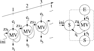
Figure 1: Algorithm graph (infinite repetition of the matrix-vector product)

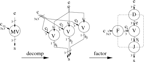
Figure 2: Subgraph MV (3 times repetition of V)

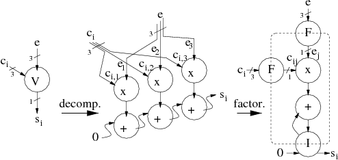
Figure 3: Subgraph V (3 times repetition of multiply-accumulate)

There are two ways for obtaining such an algorithm specification. On the one hand the user may directly input the factorized conditioned data flow graph through the graphical interface of the system level CAD software SynDEx as explained in section 4. On the other hand he may import this graph from one of the application specification languages interfaced with SynDEx, like presently one of the synchronous languages Esterel and Signal, SyncCharts a state diagram language close to Statecharts, Scicos a free software control theory oriented language close to Simulink, CamlFlow and Avs two image processing languages, and AIL close to Titus.

3.2 Architecture model

3.2.1 Multicomponent

The most typically used models for the specification of parallel or distributed computer architectures, are PRAM (Parallel Random Access Machine) and DRAM (Distributed Random Access Machine) [18]. The first model corresponds to a set of processors communicating data through a shared memory, whereas the second model corresponds to a set of processors with its own data memory (distributed memory), communicating through message passing. Although these models would be sufficient for describing the distribution (allocation) and the scheduling of the algorithm operations in the case of homogeneous architecture, they are not precise enough for dealing with heterogeneous architectures and with the distribution and the scheduling of the communications which are, as mentioned before, crucial for real-time performances. Furthermore, we also need to take into account specific integrated circuits considered as non programmable components possibly communicating with other components whatever their kinds are. The main difference between a programmable component and a non programmable component, lies in the fact that only a unique operation may be distributed (allocated) on a non programmable component, whereas on a programmable component a set of operations, which must be scheduled, may be distributed.

Thus, our heterogeneous multicomponent model [19] is an oriented graph, where each vertex is a sequential machine (automaton with output) and each edge is a connection between the output of a sequential machine and the input of another sequential machine, thus forming a network of automata [20]. There are five types of vertices: the operator for sequencing computation operations, the communicator for sequencing communication (DMA channel), the memory for memorizing data or program, and finally the bus/mux/demux (BMD) with or without arbiter for selecting from and diffusing data toward a memory. When there is an arbiter in a bus/mux/demux/arbiter, this one is also a sequential machine deciding which resource will access to a memory, which is, in this case, a shared resource. The bus/mux/demux and the memory are considered as degenerated automata. There are two types of memories: RAM memory with random access for storing data or program, and SAM with sequential access for storing data, maintaining their order, when they must be communicated from an operator or a communicator to another operator or a communicator. The different types of vertices may not be connected in whatever manner, a set of connection rules must be verified [19]. For example two operators must not be directly connected and identically for two communicators. In order to communicate data, an operator must be at least connected to a RAM or a SAM, connected in turn to another operator. When computations and communications must be decoupled, communicators must be inserted, between operator and memory, whatever its type is. Heterogeneous architecture does not only mean that vertices have different characteristics, for example different execution durations for a given operation executed on an operator or a data transfered through a communicator, but also for example, that some operations may be executed only by some specific operators, or some data must be transfered only by some specific communicators. This allows, among other possibilities related to the architecture characterization described later on in section 3.2.2, to take into account specific integrated circuits, which are only able to execute a unique operation.

A basic processor may be specified as a graph containing one operator, one data RAM, and one program RAM, all interconnected. If this processor has been designed for parallel architecture, it may also contain one or several communicators with the corresponding data RAM or SAM for communications. A direct (without routing) communication resource between two processors, may be specified as a linear graph composed of the vertices n-uple (bus/mux/demux/arbiter, RAM or SAM, bus/mux/demux/arbiter). Typically, the RAM vertex is used to model a communication by shared memory, whereas the SAM vertex is used to model a communication by message passing through a FIFO. When the computations must be decoupled from communications, some communicators must be added leading to the n-uple (bus/mux/demux/arbiter, communicator, RAM or SAM, communicator, bus/mux/demux/arbiter). A route is a path in the architecture graph connecting two operators. It is composed of a list of pairs (edge, vertex) plus an edge. A communicator allows data to cross through a processor without requiring its operator (“store and forward”). Several parallel routes may be specified in order to transfer data in parallel, but these routes may be of different length (number of elements in the route).

This model, well adapted to the optimizations presented later on in the paper, allows to specify architectures with more or less details. But it is important to be aware that the more detailed the architecture will be, the more the solution of the optimization problem will take time to be found.

The figure 4 presents the detailed model of the DSP TMS320C40 from Texas Instrument, obtained from the Data-Book [21]. Here all the connections between the vertices are bi-directional, then for the sake of readability we have represented each pair of arrows by a simple segment. The CPU, including its sequencer, its memory controller, and its arithmetic and logic unit, are represented by an operator. Since it is able to simultaneously access two internal (R0 and R1) and/or external (R_loc and R_glob) memories modeled by RAM vertices, it is connected to two bus/mux/demux (b7 and b8) which select the appropriated memory. Because these memories may also be accessed by one of the six DMA channels modeled by communicators (C1 to C6), each communicator is connected to the memories by a bus/mux/demux/arbiter (b9) which arbitrates among the communicators. Each point-to-point communication port is modeled by a SAM which may be accessed either by a DMA or by the CPU, here the operator. The operator and the communicators may access the external RAM R_loc using the arbiter of the bus/mux/demux/arbiter (b11). The operator and the communicators may access the external RAM R_glob using the arbiter of the bus/mux/demux/arbiter (b12). Each of the six bus/mux/demux (b1 to b6) selects either a SAM or the external RAM (R_glob), for each of the six communicators (C1 to C6). The bus/mux/demux (b10) selects one of the six SAM accessed by the CPU.

The figure 5 presents the model of a complex architecture composed of four TMS320C40 communicating, on the one hand by point-to-point links, and on another hand by a shared memory (R_glob). Then, although the same type of processor (operator) is used in this example, this is an heterogeneous architecture relative to the communications which are of different types. Each processor has its own local memory (R_loc).

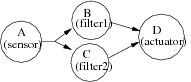
The figure 6 presents a less detailed version of the previous architecture. It is obtained by encapsulating in a unique operator the graph given in figure 4, leading to a more simple description of the architecture.

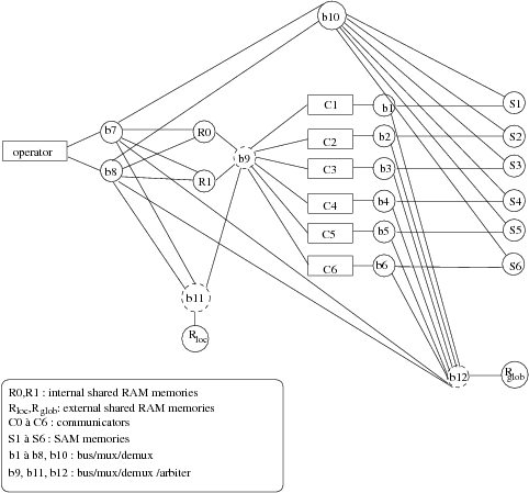
Figure 4: TMS320C40 architecture graph

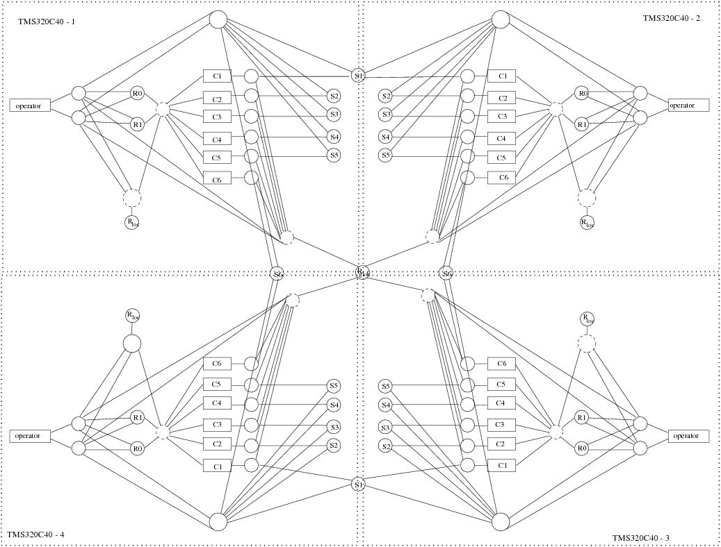
Figure 5: TMS320C40 quadri-processor architecture graph

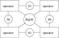
Figure 6: Simplified TMS320C40 quadri-processor architecture graph

3.2.2 Architecture characterization

The optimization process described in detail in section 3.4, is based on the multicomponent architecture characterization, meaning that to each operator and communicator, is associated the set of operations it is able to execute. Furthermore, to each operation is associated, its execution duration, the amount of memory, the power consumption, etc…, it requires. For example the CPU of a DSP is able to execute a multiply-accumulate operation in one clock cycle, and a FFT (Fast Fourrier Transform) in several cycles. Similarly, the DMA of a DSP associated to a point-to-point link is able to transfer data in a specific time, and an array of the same data in a time proportional to the number of data to transfer, plus a set-up time. The arbiter of a bus/mux/demux/arbiter has a crucial role, it is characterized by a table of priorities and a table of bandwidths which has as much elements as connected edges. The values of these elements are used to determine during the optimizations which of the operators and/or communicators will access the memory and with which bandwidth.

Each integrated circuit of the architecture is characterized separately by associating to each vertex and edge the execution duration relative to the chosen technology.

3.3 Implementation model

In this section we present how to describe all the possible implementations of a given algorithm onto a given multicomponent, in intention rather than in extension, using graph transformations. Performing an implementation is mainly a matter of reducing the potential parallelism of the algorithm according to the physical parallelism of the architecture. More precisely, it consists in distributing and scheduling the operations of the algorithm onto the architecture which has been already characterized. We use the term distribution instead of “placement” or “allocation”, which are commonly employed, in order to refer to distributed systems.

3.3.1 Distribution and scheduling

The distribution and the scheduling are formally detailed in [16]. The distribution consists in performing a partition of the initial algorithm graph, in as much elements of partition as there are of operators in the architecture graph. Then, each element of partition, i.e. each corresponding subgraph of the algorithm graph, is distributed onto an operator of the architecture graph. This amounts to label each subgraph with the name of the operator it has been distributed onto. Remember that only a unique operation may be distributed onto an operator representing a specific integrated circuit in the considered multicomponent. Then, a partition of the data dependences of the algorithm graph between operations belonging to two different elements of operations partition must be performed, in as much elements of partition as there are of routes in the architecture graph. Each element of partition, i.e. each set of corresponding data dependences of the algorithm graph, is distributed onto a route of the architecture graph. This amounts to label each set of data dependences by the name of the route it has been distributed onto. Finally, for each data dependence which connects two elements of operations partition (inter-partition edge), communication operations must be created and inserted. There are as much communication operations as there are of communicators in the route the data dependence has been distributed onto. If the route does not contain any communicator, like in a direct communication resource using a shared RAM, it is not necessary to create a communication operation. Indeed, in this case the operator performs the data transfer. Altough, the drawback is that no parallelism (decoupling) is possible between computations and communications, since the operator is also required to perform data communications. Actually, each communication operation is composed of two vertices. In the case of a SAM it corresponds to a send vertex and a receive vertex. The send is executed by the communicator which sends the data to the SAM, and the receive is executed by the communicator which receives the data from the SAM. Similarly, in the case of a RAM it corresponds to a write vertex and a read vertex.

The scheduling consists in transforming the partial order of the corresponding subgraph of operations assigned to an operator, in a total order. This “linearization of the partial order” is necessary because the operator is a sequential machine which executes sequentially the operations. Similarly, it also consists in transforming the partial order of the corresponding subgraph of communications operations assigned to a communicator, in a total order. Actually, both amount to add edges, called precedence dependences, to the initial algorithm graph.

Finally, memory allocation is also necessary in order to take into account, on the one hand the program memories used to store each operation, and on the other hand the buffers necessary to transfer data from an operation to another operation distributed onto the same operator. Then alloc vertices must also be added for each operation and for each edge in order to be distributed onto the program and the data RAM connected to the operator.

The distribution, the scheduling and the memory allocation lead to the implementation graph.

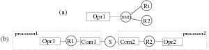
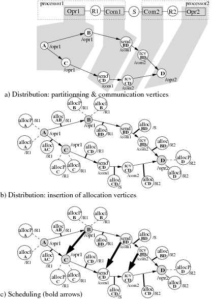
Figure 9 shows a simple implementation example of the algorithm graph presented in figure 7 onto the architecture presented in figure 8-b. Such an implementation graph is automatically generated from the results of the optimization heuristic given in the next section. In this example we want A, B and C to be executed by Opr1 and D executed by Opr2. Consequently two pairs of communication operations (send_BD, receive_BD and send_CD, receive_CD) must be inserted and associated to Com1 and Com2 in order to realize data transfers on the shared SAM S (9-a). Allocation vertices (alloc_AB, alloc_BD, alloc_AC …) have also been added in order to model all required memory allocations (9-b). Since operations B and C, which are not dependent, are distributed onto the same operator, an order of execution must be chosen between them. Notice that in this example, in order to simplify the figures, we do not take advantage of the potential parallelism between operation B and C. They should have been executed in parallel if distributed onto different operators. Thus, we add a precedence dependence edge between B and C, and a precedence dependence edge between send_BD and send_CD because they are scheduled on the same communicator Com1, and symmetrically a precedence dependence edge between receive_BD and receive_CD executed on Com2. This corresponds to the bold arrows of figure 9-c.

Figure 7: Basic example of an algorithm graph

Figure 8: Basic examples of architecture graphs

Figure 9: Example of implementation graph

Hence to summarize, the set of all the possible implementations of a given algorithm onto a given architecture may be mathematically formalized in intention, as the composition of three binary relations: namely the routing, the distribution, and the scheduling. Each relation is a mapping between two pairs of graphs (algorithm graph, architecture graph), from the set G_al × G_ar on the set G_al × G_ar. It also may be seen as an external compositional law, where an architecture graph operates on an algorithm graph in order to give as a result a new algorithm graph, which is the initial algorithm graph distributed and scheduled according to the architecture graph. In this case this is a mapping from the set G_al × G_ar on the set G_al.

Given an algorithm and an architecture graphs, there is a finite number of possible distributions and schedulings [22]. Indeed, it is possible to perform different partitions with the same number of elements (namely the number of operators), and for each subgraph assigned to an operator, it is possible to perform different linearizations, and identically for the communication operations relative to the routes and the communicators. But this leads to a very high number of possible combinations. However, it is necessary to eliminate all the schedulings which do not preserve the logical properties, remember in terms of ordering, shown with the synchronous languages as mentioned before. This amounts to preserve the transitive closure [22] of the partial order associated to the initial algorithm graph when the relation “scheduling” is applied. Moreover, the partial order of the resulting algorithm graph, which corresponds to a reduction of the potential parallelism, must be compatible with the partial order of the initial algorithm graph. Note that there is no such problem when the relation “distribution” is applied.

Our implementation model, called Macro-RTL, may be seen as an extension of the typical implementation model called RTL (Register Transfer Level) [23]. An operation of the algorithm graph corresponds to a macro-instruction (a sequence of instruction instead of one instruction) or a combinatorial circuit. A data dependence corresponds to a macro-register (several memory cells). The consumption and the production of data by an operation corresponds to a data transfer between registers through a combinatorial circuit. This model encapsulates details relative to the instructions set, the micro-programs, the pipe-line, and the cache. In that way it filters these characteristics too difficult to take into account during the optimizations. This model has a reduced complexity well adapted to the rapid optimization algorithms we aim at, however giving accurate optimization results.

3.3.2 Impact of the granularity and potential parallelism

A given algorithm offers a granularity relative to the number of operations (vertices) and data dependences (edges) it is composed of, and a level of potential parallelism relative to the lack of data dependences relative to all its possible data dependences (pairs of vertices). It is obvious that these two parameters are inter-dependent. This issue has consequences in terms of possible implementations. If the number of operations and data dependences is not sufficient enough relatively to the number of hardware resources (computation and communication sequencers), it is not possible to balance correctly the load on each resource. Similarly, if the level of potential parallelism is low, there is not enough degree of freedom when reducing the potential parallelism in order to match the physical parallelism of the architecture. On the contrary, if the number of operations and data dependences is too high, then each operation and data dependence encapsulates only few details, because in this case it has generally a low complexity, leading to a less efficient filtering of the characteristics difficult to take into account. On the other hand, the high level of potential parallelism leads to a huge number of possibilities when reducing the potential parallelism in order to match the physical parallelism. The impact of the granularity and potential parallelism is discussed in detail in [24] for an example of image processing. It is shown that an a priori choice of the granularity and potential parallelism may be modified if the real-time constraints are not satisfied. In this case, some operations must be decomposed in several operations, possibly with potential parallelism.

3.4 Optimized implementation: adequation

3.4.1 Principles

An adequation consists in searching, among all the possible implementations of the algorithm onto the architecture, for the one which corresponds to an optimized implementation relatively to the real-time and embedding constraints. The optimization problems considered in this paper, that is, the minimization of the latency and/or the cadence when the architecture is fixed, and the minimization of the architecture resources, are NP-hard problems [25].

Because it is impossible to obtain an exact solution in a reasonable time relatively to the human life, we use heuristics which are rapid enough and give a solution as close as possible to the exact (optimal) solution. In the case of complex applications involving control, signal and image processing, “rapid prototyping” is necessary. Such heuristics are well suited in order to rapidly test several variants of an implementation relatively to the cost and the availability of the hardware components, and also relatively to the addition of new functionalities. It is the reason why we first use “deterministic greedy” heuristics, i.e. no random choice and no back-tracking, and especially its “list scheduling” version because they rapidly give a result with a good precision [26]. A solution obtained with this kind of heuristics may be improved by back-tracking [27], such that the choices are modified locally or globally when elaborating a partial solution, according to the so-called “neighborhood” techniques. However, this kind of heuristics is dramatically slower. Finally, in order to improve again the quality of the solution, it may be in turn used as an initial solution for stochastic heuristics, i.e. where random choices allow to go from one solution to another one. Actually these heuristics are very slow, but are more precise mainly because they avoid local minima that the deterministic ones do not avoid. Because we are dealing with heuristics, it is also interesting to exploit the user’s skills, who is able to restrict the search space by imposing distribution or scheduling constraints in order to avoid “bad tracks” leading to local minima.

The heuristics optimizing the latency are based on the “critical paths” of the algorithm graph labeled by the durations, not only of the operations relatively to the possible operators but also of the data transfers relatively to the communication resources, whereas the heuristics optimizing the cadence are based on its “critical loops”, i.e. the cycles in the algorithm graph containing delays, leading to pipe-lining and re-timing by just moving these delays. To optimize simultaneously and independently both latency and cadence is a very difficult problem. It is the reason why usually, one is fixed while the other is intended to be optimized.

3.4.2 Example of adequation heuristics

In this section we present an efficient deterministic greedy list heuristics optimizing one latency which takes accurately into account inter-processor communications which are often neglected [28]. Its efficiency has been compared in [27] relatively to heuristics of the same family. We assume that there is only one input at the beginning and one output at the end of the algorithm graph (it is easy to transform the graph if this is not the case), and that the cadence is equal to the latency. For the sake of simplicity, we do not take into consideration the conditioning and the memory capacity. Moreover, subgraph repetitions are assumed to be entirely defactorized. The reader interested in these issues may consult [16], [19]. We have works in progress to take into account several constraints e.g. several latencies and cadences [7].

Here are the principles of the heuristics which tends to construct a global optimum from several local optima while the distribution and the scheduling are performed simultaneously. It iterates on the set O_s of schedulable operations in the algorithm graph. An operation not yet scheduled becomes schedulable when all its predecessors, excluding the delays, have already been scheduled. Initially O_s is composed of all the operations which are either input or which have only delays as predecessors. During an iteration i of the heuristics, one of the schedulable operations o and an operator p onto which this operation will be scheduled, are chosen using a cost function detailed in the next section. p belongs to the set of operators P of the architecture graph. Consequently, some successors of o become in turn schedulable. The iteration is repeated until O_s = ∅ and then, each operation has been distributed and scheduled onto an operator after a complete exploration of the initial partial order associated to the algorithm graph, thus leading to a new compatible partial order. When an operation is scheduled onto an operator after an operation which is not its predecessor, this amounts to modify the initial partial order by adding a new edge which is only an execution precedence (no data is transfered since there were no edge between both operations). If an operation o is scheduled onto an operator p and if its predecessor o′ has been scheduled onto a different operator p′, it is necessary to choose a route r, joining p and p′ (a path in the architecture graph), and to create and insert between o and o′ as much communication operations as there are of communication resources composing r, and to schedule each communication operation onto the corresponding communicator of the communication resource m. When a communication operation is scheduled onto a communication resource, this also amounts to modify the initial partial order by adding a new edge which is only an execution precedence (no data is transfered between both communication operations). It is worth noting that on each operator and on each communicator of a communication resource we obtain a total order which is compatible by construction (it is ensured that an operation is scheduled only after its predecessor) with the initial partial order. However, we obtain globally a partial order, the operations on different operators as well as the communications operations on different communicators may be executed in parallel, which is also compatible with the initial partial order. This principle guarantees that the complete execution of the operations and of the communications will never cause a deadlock.

Cost function

The goal of the heuristics consists in minimizing the latency, and here the latency is equal to the critical path of the algorithm graph labeled by the durations of the operations and of the data transfers because we only have one input at the beginning and one output at the end of the graph. The cost function is defined in terms of the start and end dates of each operation. We denote by Δ(o,p) the execution duration of the operation o belonging to the algorithm graph Gal, and by p the operator belonging to the architecture graph Gar which executes o. Γ(o) is the set of the successors of o and Γ⁻(o) the set of its predecessors. For each schedulable operation and for each operator where it is possible to distribute and schedule this operation, R the partial critical path, S(o) and E(o) (resp. S⁻(o) et E⁻(o)) the earliest start and end dates of execution from the beginning of the graph (resp. from the end of the graph), and F(o) the schedule flexibility are processed:

S(o)

max

x∈Γ⁻(o)

E(x) (or 0 if Γ⁻(o)=∅)

E(o)

S(o)+ Δ(o,p)

E⁻(o)

max

x∈Γ(o)

S⁻(x) (or 0 if Γ(o)=∅)

S⁻(o)

E⁻(o) + Δ(o)

max

o ∈ Gal

E(o) =

max

o ∈ Gal

S⁻(o)

F(o)

R − E(o) − E⁻(o)

Note the symmetry in the formulas, the dates are processed relatively to opposite directions and origins: min_{o ∈ Gal} S(o) = 0 = min_{o ∈ Gal} E⁻(o). Note also that, often in the literature [29] S=ASAP and R−S⁻=ALAP. The schedule flexibility F(o) represents the freedom degree of an operation, i.e. a time interval inside which o may be executed without increasing the critical path.

When the heuristics considers an operation o, all its predecessors have already been distributed and scheduled, but no successor has already been scheduled. Then, when E⁻ and S⁻ are processed Δ must be defined independently of all operators. The execution duration of an operation o which is not yet scheduled is defined as the arithmetic mean of all its possible execution durations on the set K(o) of the operators able to execute o:

K(o)={p∈ Gar | Δ(o,p) is defined}

Δ(o)=

Card(K(o))

∑

p∈ K(o)

Δ(o,p)

When an operation o is scheduled onto an operator p, it is scheduled after all the operations previously scheduled onto p, its execution duration Δ(o) becomes Δ(o,p) , and for each predecessor o′ of o scheduled onto an operator p′≠ p, communication operations must be created and inserted between o and o′. These communication operations must also be distributed and scheduled. Consequently, S(o) as well as the critical path R will have greater or equal values (when no communication is necessary) but never smaller, becoming S′(o) and R′ in order to indicate that communications may have been taken into account.

The cost function σ(o,p) called the schedule pressure is the difference between the schedule penalty P(o)=R′−R (critical path increase) and the schedule flexibility F(o) before the critical path increases:

σ(o,p) = P(o) − F(o) = S′(o) + Δ(o,p) + E⁻(o) − R

σ(o,p) is an improved version of the commonly used cost function F(o) which is extended by P(o). Indeed, when S′(o) (taking into account possible communications) increases, o becoming more and more critical F(o) decreases until being null and then remains null. P(o) which until now was null begins to increase. Finally σ(o,p) which is the composition of F(o) and P(o), is a function which increases continuously. Note that F(o) depends on R′ (taking into account possible communications) which may be different at each iteration of the heuristics, whereas σ(o,p) does not depend on R which remains the same whatever the iteration is. Then, it is not necessary to process the value of R at each iteration.

Choice of the best operator

The best operator p_m(o) for a schedulable operation o is either the operator on which, the user has constrained the operation to be executed (distribution constraints), or the operator which gives the smallest schedule pressure, i.e. the greater schedule flexibility and the smaller schedule penalty (increase of critical path). If several operators lead to the same results one of them is randomly chosen:

∃ p_m(o) | σ(o,p_m(o))=

min

p ∈ Gar

σ(o,p)

On the other hand, the schedulable operation which is the most urgent to schedule onto its best operator, is the operation with the greatest schedule pressure, unless its start date is greater than the date of another schedulable operation which can be executed before. It is the reason why practically it is necessary to restrict O_s to:

O_s′ = {o′ ∈ O_s | S_m(o′)<

min

o ∈ O_s

E_m(o)}

where S_m(o) and E_m(o) are the respective values of S(o) and E(o) for o scheduled onto its best operator p_m(o).

Finally, the operation chosen at each iteration is o_m such as:

∃ o_m | σ(o_m,p_m(o_m)) =

max

o ∈ O_s′

σ(o,p_m(o))

If several operations lead to the same results one of them is randomly chosen. The chosen operator is p_m(o_m) the best operator on which o_m is scheduled.

Creation, distribution and scheduling of communications

When an operation o is scheduled onto an operator p, each data dependence between this operation and one of its predecessors o′∈Γ⁻(o) already scheduled onto an operator p′≠ p, is an inter-operator data dependence. For each of these dependences, it is necessary to choose a route which will support the transfer of the data produced by o′ in the local memory of p′ to the local memory of p in order to be consumed by o. The transfer is achieved through the different communication resources composing the route.

The number of possible routes (path in the architecture graph) may be large for complex architectures, and consequently the choice of the best route may take a very long time because it is necessary to compare, for a data dependence to transfer, all the possible cases of distribution and scheduling in all the communicators of the route. In order to reduce this time the heuristics performs an incremental choice using routing tables. This method is described in details in [28]. Briefly, for each operator the shortest routes (minimum number of communication resources) between this operator and all the other operators, is determined. These shortest routes and the first communication resource of this route are memorized in its routing table. If there are several possible routes between two operators with the same minimum number of communication resources, these routes, called parallel routes, are memorized. Then, each time the heuristics has to evaluate the cost of an inter-operator data dependence, for each operator of the route (p′,p) it chooses in the routing table among the possible first communication resource m of the shortest routes from this intermediate operator and p, the one which first completes the communication operation c. This communication operation may be either another communication operation which has been previously scheduled onto m because it has to transfer the same data (this is the case of a data diffusion using the same first part of the route), or c is a new communication operation that must be created and inserted in the algorithm graph between the previous communication operation in the route (or o′ at the beginning of the route) and o. c must be scheduled onto m by adding a precedence dependence between the last communication operation scheduled onto m before c, and c. The heuristics proceeds like this until p is reached. This approach allows to take into account on the one hand parallel routes in order to balance the load of the communication resource, and on the other hand the possibilities to reuse already routed communications avoiding to needlessly duplicate communications.

3.4.3 Resources minimization

In the previous section we assumed that the architecture graph is given and then, all the resources like operators, communicators, etc, are also given, as well as the way they are interconnected. In this case we aim at exploiting the architecture resources as good as possible. However, in some cases it is possible to decrease the number of resources while satisfying the real-time constraints. Therefore, an iterative process may be set up, where the user tries to decrease the number of resources and verifies if the real-time constraints are still met.

3.5 Executives generation

Here, we only present the main principles of the executives generation for multicomponent architecture. The code executable in real-time, is the result of an ultimate graph transformation of the implementation graph obtained after the optimized distribution and scheduling described previously. The graph transformation and the obtained code are detailed in [19, 30].

As soon as a distribution and a scheduling have been chosen, that is to say determined “off-line”, it is possible to automatically generate dedicated real-time distributed executives. They are mainly static with a dynamic part only for taking into account conditionings which depends of test values only known when the application is executed in real-time. From the same informations, it is also possible to configure the fixed priorities of a set of tasks scheduled by a standard RTOS, like: Vrtx, Irmx, Virtuoso, Lynx, Osek, RT-Linux, etc... However, this approach although it should allow the use of COTS (Component Of The Shelf) which may reduce costs, will obviously decrease the performances by increasing the overhead of the executives. Note that in both cases we use an “off-line” approach, well suited to real-time applications which need to be deterministic.

The dedicated executives are mainly based on the one hand on the sequencing, possibly conditioned, of the algorithm operations distributed on a particular processor, and on the other hand on an inter-component communications system without any deadlock by construction, ensuring a global synchronization between all the operations running on different processors. This is the reason why we chose the name SynDEx, acronym for Synchronized Distributed Executives, for the system level CAD software presented in section 4 which implements the AAA methodology. Deadlocks due to data dependence cycles are detected during the algorithm graph specification and during the graph transformations, taking into account the architecture graph, and leading to the implementation graph.

The algorithm graph specified by the user, possibly through a high level language (perhaps performing verifications), is transformed during the optimized distribution and scheduling, avoiding cycles since its partial order is reinforced without introducing any cycle. Similarly, the implementation graph is also transformed in order to produce the executives, by adding to the implementation graph new vertices and their corresponding edges. In order to satisfy the real-time characteristics of the algorithm, each executive includes an infinite repetition due to the reactive nature of the applications, and synchronizations which ensure that the data communications will be executed, without any deadlock, according to the scheduling chosen by the optimization heuristics. This preserves the logical properties shown with the high level specification languages when some are used. The synchronization operations guarantee execution precedence between computation operations and communication operations belonging to different sequences, sharing data in mutual exclusive access. Each synchronization operation uses a semaphore automatically generated. In [19] it is shown with Petri nets that these semaphores allow the executives to verify the partial order of the initial algorithm graph.

There are as many generated executives as there are of processors. Each executive file is a macro-code which is independent of the processor type. It is composed of a list of macros which will be translated by a macro-processor, for example the Gnu tool “m4”, using the appropriate definitions of macros, into a source program (C, assembler, etc...). Then, each of these source programs will be compiled and linked, and finally loaded and executed on the target processor in order to run in real-time. The definition macros which are dependent of the processor, are of two types. The first one is an extensible set of application definition macros describing the operations behavior, e.g. an addition or a filter. The second one is a fixed set of system definition macros describing the application support: loading and initialization of program memory, management of data memories, sequencing (conditional and unconditional branchings respectively for conditionings, and finite and infinite loops), inter-processor data communications (send, receive, write, read), synchronization inside a processor between a sequence of computations and one or several sequences of communications, synchronization between sequences of communications belonging to different processors, and finally chronometric recording for operations and data transfers characterization. This latter set of definition macros is called the executive kernel and one is needed by processor.

The process of the executives generation is perfectly systematic. It automates the work performed by hand by a system programmer, leading to a very low overhead even though they are automatically generated.

The executives generation is performed following four steps [19]: (1) transformation of the optimized implementation graph into an execution graph, (2) transformation of the execution graph into as many macro-code as there are of processors, (3) transformation of each macro-code into a source file, (4) compilation, download and execution of each source file.

3.5.1 From implementation graph to execution graph

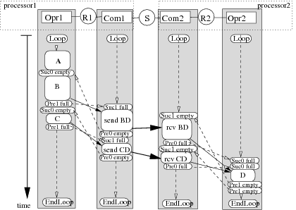
This transformation consists in adding new types of vertex: Loop, EndLoop and pre-full/suc-full, pre-empty/suc-empty vertices. This is done following two steps:

since the considered applications are reactive (i.e. they are in constant interaction with the environment that they control) the sequence of operations distributed onto each operator must be infinitely repeated. For each sub-graph of the algorithm distributed onto an operator a Loop vertex is added and connected before the first operation of the sequence, and a EndLoop vertex is added and connected after the last operation (Cf. figure 12),
when two operations distributed onto two different operators are data dependent, a communication must be performed between these operators. The operator which executes the producing operation must cooperate with a communicator in order to send (resp. write) the data to a SAM (resp. a RAM), symmetrically another communicator must cooperate with the operator which executes the consuming operation in order to receive (resp. read) the data from the SAM (resp. the RAM). When considering one infinite repetition, for each pair operator-communicator, operator and communicator must be synchronized because both these sequencers share the data to send. 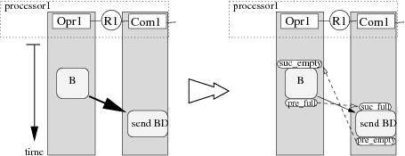This synchronization is necessary in order to carry out the inter-partition edge, represented by a bold arrow on figure 10. It is implemented on processor1 by replacing this edge with a linear sub-graph made of an edge connected to a pre-full vertex which is itself connected to a suc-full vertex (right part of figure 10). The pre-full (resp. suc-full) vertex is allocated on the same partition as the producing (resp. consuming) operation of the initial inter-partition edge. Pre-full and suc-full vertices are operations able to read-modify-write a binary semaphore allocated into the memory shared by the two sequencer partitions. If suc-full (which precedes the send operation) is executed before the connected pre-full (which follows the operation B) then the suc-full waits for the end of the pre-full execution which signals that the buffer containing the value produced by the operation B is full. This mechanism ensures a correct execution order between the execution of the operation B and the operation send BD which sends the value produced by B to the operation D executed on another processor2. When considering two consecutive infinite repetitions, it is also necessary to avoid that a producing operation overwrites the data which has not yet been sent. For this purpose a pair of suc-empty, pre-empty vertices is inserted. Pre-empty is inserted after the consuming operation send BD while suc-empty is inserted before the producing operation B. Pre-empty signals that the sent of the data produced by B during the previous repetition was terminated.
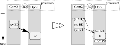
Symetrically, on processor2 which receives and consumes with operation D the result produced by operation B executed on processor1, the synchronization represented by a bold arrow on figure 11 is implemented by replacing this edge with a linear sub-graph made of an edge connected to a pre-full vertex which is itself connected to a suc-full vertex (right part of figure 11). Similarly, when considering two consecutive infinite repetitions, a pre-empty is inserted after the consuming operation D while suc-empty is inserted before the producing operation rcv BD .
Notice that when a SAM is used to transfer the data between the communicators, no other synchronizations is necessary since this type of memory ensures an hardware write-read synchronization. In the case of a RAM, a synchronization, similar to the one between operator and communicator, must be added.

Figure 12 depicts a complete example of the execution graph obtained after the transformation of the implementation graph given in figure 9. Loop/EndLoop vertices have been added on Opr1,Com1,Com2 and Opr2 operations. In order to simplify the graph, allocation vertices are not represented.

Figure 10: Principle of synchronization send

Figure 11: Principle of synchronization rcv

Synchronization operations are fundamental in distributed systems since they guarantee that each data-dependence of the algorithm graph is implemented correctly. They guarantee that all buffers, storing the data, are always accessed in the order specified by the data-dependences in a way that this order is satisfied at runtime independently of the execution durations of the operations. Moreover, they guarantee that no data is lost. Therefore, the implementation optimization, even if it may be biased by inaccurate architecture characteristics, is safe in the sense that it cannot induce, unlike human programmers, runtime synchronization errors (such as deadlocks, or lost data). Indeed, such synchronizations are usually hand-written inside the application code such that deadlocks may occur if the designer misses one of them or does not write them in the the correct order. Finally, since synchronization operations are added in order to guarantee the partial execution order specified in the initial algorithm graph, and because the implementation of our synchronization reflects exactly our models, we do not have trouble due to run-time overhead (as consensus waiting problem) induced by synchronization. The run-time overhead induced by the synchronizations is completely mastered and its cost can be taken precisely into account by the optimization heuristics. The proposed technique allows big savings thanks to a minimization of the coding process which actually is reduced to the one of the application operations. In addition, it leads to a minimum debugging time.

Figure 12: Execution graph after transformation of implementation graph of figure 9

3.5.2 From execution graph to macro-code

Once the executive graph has been built, the sub-graph distributed onto each operator (processor) of the architecture graph, is transformed into a sequence of macro-instructions. The use of a macro-code enables to mix easily different programming languages (C, Fortran, assembler, SystemC…) that can be found in heterogeneous architecture.

The macro-code structure for an operator opr is sequentially composed of:

macros allocating semaphores and buffers for each allocation vertex allocated to each RAM connected to opr we generate an alloc_(name) macro. name is generated from the operation name producing the data,
as many communication sequences as existing communicators connected to opr (only one communicator is connected to each operator in our example). This sequence is generated between a pair of ComThread_, EndComThread_ macros. Such a sequence is built by exploration of the sequence of totally ordered vertices allocated to the communicator partition. For each vertex of the sequence we generate a corresponding macro (send_, receive_, read_, write_, pre_full, suc_full, pre_empy, suc_empty). In order to distinguish a pair (pre_, suc_) synchronizing a sequence of communications with a sequence of computations from a pair (pre_, suc_) synchronizing a sequence of computations with a sequence of communications, we use a pair (pre0_, suc0_) for synchronizing a sequence of communications with a sequence of computations, and a pair (pre1_, suc1_) for synchronizing a sequence of computations with a sequence of commmunications. The arguments of these macros are computed from the edges connected to their corresponding vertices.
a unique computation sequence. This sequence is generated between a pair of Main_, EndMain_ macros. Such a sequence is also built by exploration of the sequence of totally ordered vertices allocated to the operator partition. A spawn_thread_(com1) macro has in charge to run the communication thread com1. This thread is executed under DMA interrupt (end of transfers interrupt) of the main thread.

In order to generate an executable code whose partial order is consistent with the implementation graph, it is important to remember that the translation/print process follows exactly the order given to the vertices distributed onto this operator.

In order to measure the real-time performances of an application carried out with the AAA methodology, it is possible to generate executives with chronometric operations automatically inserted before each computation and each data communication. The real-time performances measure are performed in two steps: first on each processor the real-time start and end dates are measured and memorized using the real-time clock of the processor, second at the end of the application all the memorized values are transfered to one of the processors with mass storage capabilities. These measures may be compared to those computed by the heuristics in order to determine the optimized distribution and scheduling. The difference between the real-time measures and the computed measures, is representative of the difference between the models used in AAA and the reality. Moreover, these measures allow to determine the execution duration of the operations and data transfers, necessary to perform the architecture characterization as described in section 3.2.2.

3.5.3 Macro-code to source files

Each macro-code is translated by a macro-processor into a source code depending on the language chosen for the target operator. We use the free software Gnu-m4 macro-processor (http://www.gnu.org/software/m4).

A macro is translated either into a sequence of in-lined instructions, or into a call to a separately compiled function. These macros are classified in two sets corresponding to two kinds of libraries. The first one is an extensible set of application macros, which support the algorithm operations. The second, constituting an executive kernel, is a fixed set of system macros, which support code downloading, memory management, sequence control, inter-sequence synchronization, inter-operator transfers, and runtime timing (in order to characterize algorithm operations and to profile the application).

Once the executive libraries have been developed for each type of processor, it takes only few seconds to automatically generate, compile and download the deadlock free code for each target processor of the architecture. It is then easy to experiment different architectures with various interconnection schemes.

3.5.4 Example of macro-code

Figure 13 is an example of code generation obtained by transformation of the execution graph given in figure 12. This example will focus on processor p1 (the code of processor p2 given in figure 14 is generated symmetrically):

generation of a semaphores_ macro (lines 5-10) which allocates all the necessary semaphores, one pair _full _empty for each communication. The semaphores are managed by pre_ and suc_ synchronization operations;
generation of alloc_ macros (lines 11-14) for each allocation vertex associated to RAM R1 of figure 9 (the reader must remind that for readability allocation vertex are not drawn on figure 12);
the unique communicator sequence is generated between a pair of thread_(SAM,x,p1,p2) and endthread macros (lines 15 to 28), where SAM is the type of the communication, x is the name of the communication gate, p1,p2 are the communicating processors. Each communication vertex scheduled on the communicator com1 is translated into a send_ (lines 21 and 24) or a recv_ macro. Each synchronization vertex is translated into the corresponding macros pre_(empty/full) and suc_(empty/full) in order to synchronize the communicator sequence with the operator sequence, and vice-versa the operator sequence with the communicator sequence. The pair (pre1_(full), suc1_(full)) (lines 36 and 20) synchronizes the operator sequence with the communicator sequence in the same repetition, whereas the pair (pre0_(empty), suc0_(empty)) (lines 22 and 34) synchronizes the communicator sequence of the current repetition with the operator sequence of the previous repetition to guarantee that the send (line 21) in the previous repetition is terminated;
the unique operator opr1 sequences its operations between a pair of main_ and endmain_ macros (lines 29 to 43). Each operation vertex is translated into a macro with the same name A, B, C (lines 33, 35 and 38) taking the allocation vertice names as argument.

Then, theses files are translated into the language of the target processor by the Gnu-m4 macro-processor using a processor specific library containing the macro-definitions of each system macro, and the macro-definitions of each application operation.

3.5.5 Example of macro-definition

Below is an example of macro-definition used by the macro-processor Gnu-m4 to translate SynDEx macro-instruction alloc_ into C code.

Consider the macro-instruction:

   alloc_(int,x,3)

To produce C code the definition of this macro is performed in two steps:

First step: (in syndex.m4x, standard library)

def(`alloc_',
        define(`$2_type_', $1)dnl
        define(`$2_size_', ifelse($3,,1,$3))dnl
        ifdef(`$1_alloc_', `$1_alloc_', `basicAlloc_')')($2)')

Second step: (in U.m4x library, C-Unix specific library)

define(`basicAlloc_', `_($'`1_type_ _$'`1[$'`1_size_];)

Consequently, the result given by Gnu-m4 for the above macro-instruction is:

   int x[3];

Similarly, the translation of a send_ macro may be DMA_config_write_(alloc_BD,size_of(alloc_BD), com2) if com2 is the addresses of a RAM writable by a DMA channel of the processor. The implementation of synchronization macros is generally coded in assembly language, since performance and context switching minimization between the communication sequences and the computation sequence are required.

-1cm

01: include(syndex.m4x)dnl                          ; Include generic kernel
02: dnl
03: processor_(proc,p1,al,                          ; START FILE p1.m4
04: SynDEx-7.0.2 (C) INRIA 2001-2009, 2009-10-07 10:33:55)
05: semaphores_(                                    ; Semaphores declarations
06:  Semaphore_Thread_x,
07:  _al_C_CD_p1_x_empty,
08:  _al_C_CD_p1_x_full,
09:  _al_B_BD_p1_x_empty,
10:  _al_B_BD_p1_x_full)
11: alloc_(int,_al_A_AB,1)                          ; Buff declarations
12: alloc_(int,_al_A_AC,1)
13: alloc_(int,_al_B_BD,1)
14: alloc_(int,_al_C_CD,1)
15: thread_(SAM,x,p1,p2)                            ; START SEQ COMMUNICATIONS
16:   loadDnto_(,p2)
17:   Pre0_(_al_B_BD_p1_x_empty,,_al_B_BD,empty)
18:   Pre0_(_al_C_CD_p1_x_empty,,_al_C_CD,empty)
19:   loop_
20:     Suc1_(_al_B_BD_p1_x_full,,_al_B_BD,full)    ; Wait for buff BD full
21:     send_(_al_B_BD,proc,p1,p2)                  ; Send buff BD p1 -> p2
22:     Pre0_(_al_B_BD_p1_x_empty,,_al_B_BD,empty)  ; Signal buff BD empty
                                                    ; in current repetition
23:     Suc1_(_al_C_CD_p1_x_full,,_al_C_CD,full)    ; Idem as send buff BD
24:     send_(_al_C_CD,proc,p1,p2)
25:    Pre0_(_al_C_CD_p1_x_empty,,_al_C_CD,empty)
26:   endloop_
27:   saveFrom_(,p2)
28: endthread_                                      ; END SEQ COMMUNICATIONS
29: main_                                           ; START SEQ COMPUTATIONS
30:   spawn_thread_(x)                              ; Launch comm thread
31:   A(_al_A_AB,_al_A_AC)
32:   loop_
33:     A(_al_A_AB,_al_A_AC)                        ; Compute A (sensor)
                                                    ; write result in buff
                                                    ; AB and AC
34:     Suc0_(_al_B_BD_p1_x_empty,x,_al_B_BD,empty) ; Wait for buff BD empty
                                                    ; in previous repetition
35:     B(_al_A_AB,_al_B_BD)                        ; Compute B read in buff
                                                    ; AB write in buff BD
36:     Pre1_(_al_B_BD_p1_x_full,x,_al_B_BD,full)   ; Signal buff BD full
                                                    ; allowing send BD
37:     Suc0_(_al_C_CD_p1_x_empty,x,_al_C_CD,empty) ; Idem as compute B
38:     C(_al_A_AC,_al_C_CD)
39:     Pre1_(_al_C_CD_p1_x_full,x,_al_C_CD,full)
40:   endloop_
41:   A(_al_A_AB,_al_A_AC)
42:   wait_endthread_(Semaphore_Thread_x)           ; Wait end comm threads
43: endmain_                                        ; END SEQ COMPUTATIONS
44: endprocessor_                                   ; END FILE p1.m4

Figure 13: Macro-code corresponding to the algorithm graph of figure 9 for processor p1

-1cm

include(syndex.m4x)dnl
dnl
processor_(proc,p2,figure9,
SynDEx-7.0.2 (C) INRIA 2001-2009, 2009-10-07 10:33:55)

semaphores_(
  Semaphore_Thread_x,
  _al_C_CD_p2_x_empty,
  _al_C_CD_p2_x_full,
  _al_B_BD_p2_x_empty,
  _al_B_BD_p2_x_full)

alloc_(int,_al_B_BD,1)
alloc_(int,_al_C_CD,1)

thread_(SAM,x,p1,p2)
  loadFrom_(p1)
  loop_
    Suc1_(_al_B_BD_p2_x_empty,,_al_B_BD,empty)
    recv_(_al_B_BD,proc,p1,p2)
    Pre0_(_al_B_BD_p2_x_full,,_al_B_BD,full)
    Suc1_(_al_C_CD_p2_x_empty,,_al_C_CD,empty)
    recv_(_al_C_CD,proc,p1,p2)
    Pre0_(_al_C_CD_p2_x_full,,_al_C_CD,full)
  endloop_
  saveUpto_(p1)
endthread_

main_
  spawn_thread_(x)
  D(_al_B_BD,_al_C_CD)
  Pre1_(_al_B_BD_p2_x_empty,x,_al_B_BD,empty)
  Pre1_(_al_C_CD_p2_x_empty,x,_al_C_CD,empty)
  loop_
    Suc0_(_al_B_BD_p2_x_full,x,_al_B_BD,full)
    Suc0_(_al_C_CD_p2_x_full,x,_al_C_CD,full)
    D(_al_B_BD,_al_C_CD)
    Pre1_(_al_B_BD_p2_x_empty,x,_al_B_BD,empty)
    Pre1_(_al_C_CD_p2_x_empty,x,_al_C_CD,empty)
  endloop_
  D(_al_B_BD,_al_C_CD)
  wait_endthread_(Semaphore_Thread_x)
endmain_

endprocessor_

Figure 14: Macro-code corresponding to the algorithm graph of figure 9 for processor p2