Chapter 8 Example 8: a complete realistic application from adequation to execution

From the principal window, choose File / Save as and save your eighth application under a new folder of yout tutorial folder (e.g. my_example8) with the name example8.

8.1 The aim of the example

In the seven previous examples we have learnt how to use SynDEx’s GUI to create architectures, algorithms, launch adequation, obtain executive files... Now, we have sufficient knowledge to perform a simple automatic control application that will be executed on a multiprocessor architecture.

First the application is described and the system is defined in Scicos (the block diagram editor of the Scilab software¹). Second the corresponding SynDEx application is created (using the Example 1 to 3 of the tutorial). This needs the generation of some C code following the method discussed in Example 7. Finally, we compile the application to obtain executable for several processors as it has been shown in Examples 6 and 7. SynDEx generates the code necessary to the communication between the processors.

8.2 The model

We consider a system of two cars. The second car C₂ follows the car C₁ trying to maintain the distance l while the acceleration and the deceleration of C₁. We call: x₁(t) the position of the first car; x₂(t) the position of the second car plus l; x_1(t) and x_2(t) the speeds of two cars. We denote k₁ and k₂ the inverse of the car masses. We call r(t) the reference speed chosen by the first driver. We suppose that we are able to observe the speed of the first car and the distance between the cars.

We have the following fourth order (four degrees of liberty) system:

x₁= k₁ u₁ x₂= k₂ u₂ y₁= x_1 y₂= x₁ − x₂ (1)

We will decompose the system into mono-input mono-output system S₁ (u₁,y₁) and S₂ (u2,y2). Denoting by uppercase letter the Laplace transform of the variables, we have Y₁=k₁ U₁/s and Y₂=(k₁ U₁ − k₂ U₂)/s² where U₁ is seen as a perturbation that we want reject in the second system.

A first proportional feedback U₁=ρ₁(R−Y₁) will insure the first car to follow the reference speed. The second controller will be proportional derivative U₂=ρ₂ Y₂+ρ₃ s Y₂ (in fact we will suppose in the following diagram that the derivative of y₂ is also observed). The coefficient ρ₁ is obtained by placing the pole of the first loop:

Y₁=ρ₁k₁R/(s+ρ₁k₁).

The coefficient ρ₂ and ρ₃ are obtained by placing the pole of the transfer from U₁ to Y₂ in the closed loop system which is given by:

Y₂=U₁k₁/(s²+k₂ρ₃s +k₂ρ₂).

8.3 The controllers

The purpose of the controller of the C₁ car is to follow the reference in speed given the first driver. It stabilizes the C₁ speed around its reference speed by using pole placement. For example, gains are respectively: (0, -5, 0, 0, -5). The controller of second car stabilizes the distance between the two cars. It stabilizes y₂ around 0 by pole placement. For example, gains are respectively: (4, 4,-4,-4).

The controler of C₂ knows these informations and sends them electronically to C₁. This remark is available for C₁.

8.3.1 Block diagrams of controllers

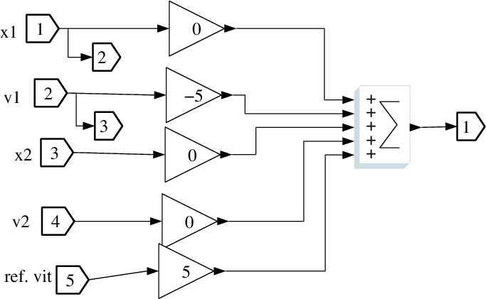
Figure 8.1: Scicos controller of the first car

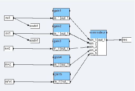
Figure 8.2: SynDEx controller of the first car

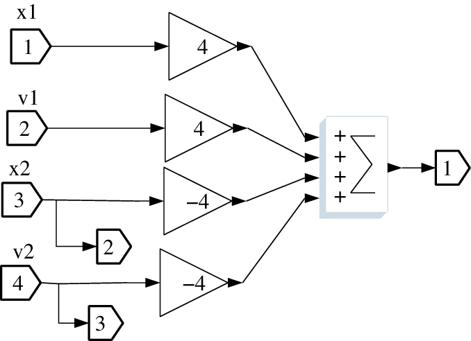
Figure 8.3: Scicos controller of the second car

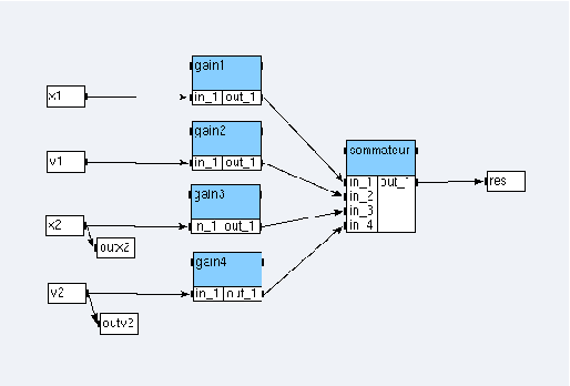
Figure 8.4: SynDEx controller of the second car

Our controllers are simple. They are represented in figures 8.1 and 8.3 in Scicos and figures 8.2 and 8.4 in SynDEx:

create a gain_def function with one input port in_1, one output port out_1 and a parameter named value. Notice that all ports will be of type float;
then create sommateur2_def, sommateur4_def, and sommateur5_def functions, respectively with two input ports (in_1 and in_2), four input ports (from in_1 to in_4), and five input ports (from in_1 to in_5). Each of these three functions is created with only one output port out_1;
finally create both algorithms controleur1_sup and controleur2_sup (cf. figures 8.2 and 8.4), setting their gain parameters respectively to 0, -5, 0, 0, 5 and 4, 4 ,-4 , -4.

8.3.2 Source code associated with the functions

We associate C source code to each function definition: gain and nary-sums. The code is inserted for the default processor.

Gain

A gain is a function that multiplies its input by a coefficient given as a parameter, named GAIN. After adding this parameter, open the code editor of the gain definition and write the following code in the loop phase of the default processor:

  
    @OUT(out_1)[0] = @IN(in_1)[0] * @PARAM(GAIN);

Sum

We have three different forms of sum depending of its arity: two, four or five input ports:

open the code editor of the sum function with two input ports and write the following code in the loop phase of the default processor:
```
    
      @OUT(out_1)[0] = @IN(in_1)[0] + @IN(in_2)[0];
    
  
```
open the code editor of the sum function with the four input ports and write the following code in the loop phase of the default processor:
```
    
      @OUT(out_1)[0] = @IN(in_1)[0] + @IN(in_2)[0] +
      @IN(in_3)[0] + @IN(in_4)[0];
    
  
```
open the code editor of the sum function with the five input ports and write the following code in the loop phase of the default processor:
```
    
      @OUT(out_1)[0] = @IN(in_1)[0] + @IN(in_2)[0] +
      @IN(in_3)[0] + @IN(in_4)[0] + @IN(in_5)[0];
    
  
```

8.4 The complete model

In a real application, our job stops with the SynDEx’s adequation of the two controllers on their associated architectures. Nevertheless, for pedagogic reasons, we will simulate the whole system (with the dynamics of the cars) in the aim to verify that our application does the same job that Scicos.

8.4.1 The car dynamics

SynDEx is only used in discrete time model (not continuous time) and is not able to manage implicit algebraic loop. That is, in SynDEx, any loop contains at least a delay 1/z. Therefore, our application which is a continuous time dynamic system described in Scicos, must be discretized in time to be used in SynDEx.

The differential equation ẋ=u is discretized using the simplest way: the Euler scheme. Let us denote by h the step of the discretization and x₀ an arbitrary initial value, the discretized system can be written as:

x_n+1 − x_n= uh (2)

Finally, the system is given in Scicos in the figure 8.5 and 2 is given in SynDEx in the figure 8.6. Notice that the variable h is stored in the Scicos context, and used in the input of the gain and the clock definition. In SynDEx, h is defined as parameter in the definition of a gain and the clock definition is directly used in the source code associated with operations.

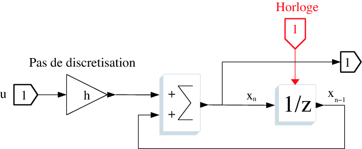
Figure 8.5: An integral discretized in Scicos

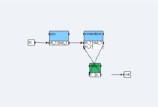
Figure 8.6: An integral discretized in SynDEx

Create the integrale_discrete_sup algorithm (cf. figure 8.6). Notice that pas is of type gain_def with parameter GAIN equal to 0.001, sommateur is of type sommateur2_def, and retard is of type float/delay<{0};1>.

The car dynamics are given with Scicos block diagrams in the figure 8.7 and with SynDEx operations in the figure 8.8, where the input 1 (ref) is the acceleration of the car. The first integral gives the speed of the car and the second its position.

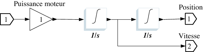
Figure 8.7: Car dynamics with Scicos block diagrams (continous time)

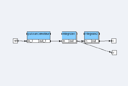
Figure 8.8: Car dynamics with SynDEx operations

Create the mecanique_sup algorithm (cf. figure 8.8). Notice that puissancemoteur is of type gain_def with parameter GAIN equal to 1 whereas integrale1 and integrale2 are of type integrale_discrete_sup.

8.4.2 The cars and their controllers

In the following diagrams (from 8.9 to 8.12), the blocks (operations) denoted by meca are the car dynamics. Let us get the controllers of the two cars.

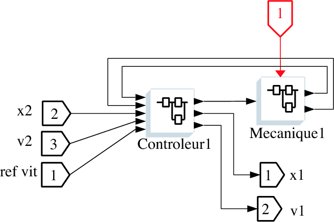
Figure 8.9: Scicos C₁ car dynamics and its controller

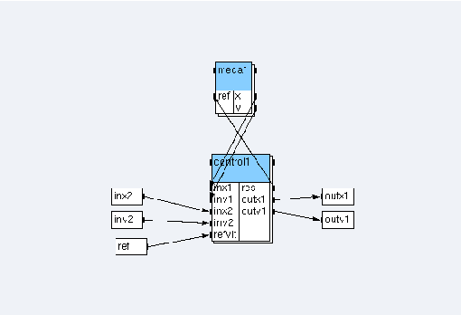
Figure 8.10: SynDEx voiture1_sup car dynamics and its controller

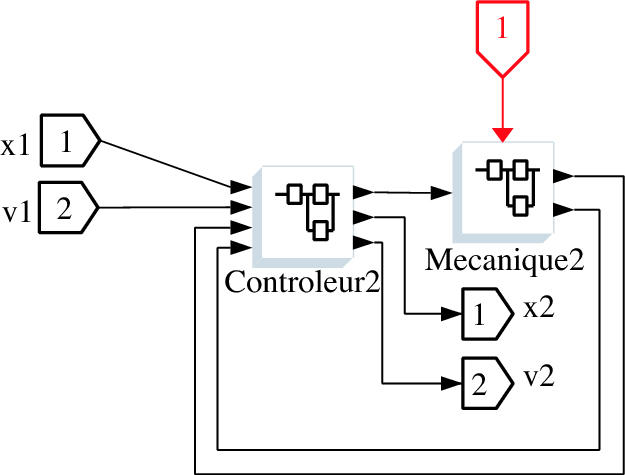
Figure 8.11: Scicos C₂ car dynamics and its controller

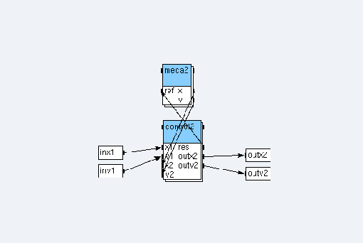
Figure 8.12: SynDEx voiture2_sup car dynamics and its controller

Create the voiture1_sup and voiture2_sup algorithms (cf. figures 8.10 and 8.12). Notice that meca1 and meca2 are references to mecanique_sup whereas control1 (resp. control2) is a reference to controleur1_sup (resp. controleur2_sup).

8.4.3 The main algorithm

Create the following definitions (definitionName<PARAM>):

senseur_def<POSI_ARRAY> with one output port out_1,
vitesse_def<POSI_ARRAY> with one input port in_1,
scope_def<POSI_ARRAY> with two input ports in_1 and in_2.

Then create algomain. Create the reference speed ref_vit of definition senseur_def<0>, the reference vitesse x_1 of definition vitesse_def<1>, the reference distance between the two cars of definition scope_def<2>, the reference vehicule1 of definition voiture1_sup and the reference vehicule2 of definition voiture2_sup, connect them according to the figure 8.13.

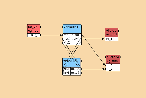
Figure 8.13: Main algorithm

8.4.4 Source code associated with the sensor and the actuator

We associate C source code to each function definition: input and two kinds of output.

Input

In our Scicos application an input is a square wave generator. As a rule, we will simulate a square wave generator by reading values in a text file (named ref_vitesse.txt). We will use the fopen, the fclose and the fscanf functions (stdio.h library). We will also use assertions (assert.h library) to ensure that the opening of a file has been successful.

For the moment, let suppose that it exists an array of FILE* (the structure returned by the fopen function) called fd_array and a variable called timer to simulate a pseudo-timer. Our sensor has a parameter called POSI_ARRAY to remember the position of the FILE* structure in the array.

Now, open the code editor of the senseur_def sensor and write the following code in the init phase of the default processor:

  
    timer = 0;
    fd_array[@PARAM(POSI_ARRAY)] = fopen("ref_vitesse.txt", "r");
    assert(fd_array[@PARAM(POSI_ARRAY)] != NULL);

In the Scicos application, we have defined the clock period of the square wave generator to the value 5 and the step of discretization h to the value 0.001. Thus we need, in the SynDEx application, to send 5000 times the same value. To count, we use the variable timer. All the 5000-th times, we read a new value in the file.

Write the following code in the loop phase of the default processor:

  
    timer = (timer + 1) % 5000;
    if (timer == 1)
    fscanf(fd_array[@PARAM(POSI_ARRAY)], "%f\n", &data);
    @OUT(out_1)[0] = data;

We need to free memory by closing the file. Write the following code in the end phase of the default processor:

  
    fclose(fd_array[@PARAM(POSI_ARRAY)]);

Speed output

An output saves in a file the values of the system states. Thus, an output has a parameter called POSI_ARRAY to remember the position of the array where the stream has been saved. Open the code editor of the vitesse_def actuator and write the following code in the init phase of the default processor:

  
    fd_array[@PARAM(POSI_ARRAY)] = fopen("actuator_@TEXT(@PARAM(POSI_ARRAY))", "w");
    assert(fd_array[@PARAM(POSI_ARRAY)] != NULL);

The loop phase, allows to save the values:

  
    fprintf(fd_array[@PARAM(POSI_ARRAY)], "%E\n", @IN(in_1)[0]);

We need to free the memory by closing the file. Write the following code in the end phase:

  
    fclose(fd_array[@PARAM(POSI_ARRAY)]);

Distance output

Contrary to the first type of output, this output has two input ports but the init and end source codes are identical. The loop phase differs. Open the code editor of the scope_def actuator and write the following code in the init phase of the default processor:

  
    fprintf(fd_array[@PARAM(POSI_ARRAY)], "%E\n", (@IN(in_1)[0] - @IN(in_2)[0]));

8.4.5 The `example8_sdc.m4x`

SynDEx’s code generation will create the example8_sdc.m4x file (as explained in Example 7):

  
    define(‘example8_algomain’,‘algomain’)
    define(‘algomain’,‘ifelse(
    processorType_,processorType_,‘ifelse(
    MGC,‘INIT’,“”,
    MGC,‘LOOP’,“WARNING: empty code for macro $0 in loop phase”,
    MGC,‘END’,“”)’)’)

    define(‘example8_controleur1_sup’,‘controleur1_sup’)
    define(‘controleur1_sup’,‘ifelse(
    processorType_,processorType_,‘ifelse(
    MGC,‘INIT’,“”,
    MGC,‘LOOP’,“WARNING: empty code for macro $0 in loop phase”,
    MGC,‘END’,“”)’)’)

    define(‘example8_controleur2_sup’,‘controleur2_sup’)
    define(‘controleur2_sup’,‘ifelse(
    processorType_,processorType_,‘ifelse(
    MGC,‘INIT’,“”,
    MGC,‘LOOP’,“WARNING: empty code for macro $0 in loop phase”,
    MGC,‘END’,“”)’)’)

    define(‘example8_gain_def’,‘gain_def’)
    define(‘gain_def’,‘ifelse(
    processorType_,processorType_,‘ifelse(
    MGC,‘INIT’,“”,
    MGC,‘LOOP’,“WARNING: empty code for macro $0 in loop phase”,
    MGC,‘END’,“”)’)’)

    define(‘example8_integrale_discrete_sup’,‘integrale_discrete_sup’)
    define(‘integrale_discrete_sup’,‘ifelse(
    processorType_,processorType_,‘ifelse(
    MGC,‘INIT’,“”,
    MGC,‘LOOP’,“WARNING: empty code for macro $0 in loop phase”,
    MGC,‘END’,“”)’)’)

    define(‘example8_scope_def’,‘scope_def’)
    define(‘scope_def’,‘ifelse(
    processorType_,processorType_,‘ifelse(
    MGC,‘INIT’,“”,
    MGC,‘LOOP’,“WARNING: empty code for macro $0 in loop phase”,
    MGC,‘END’,“”)’)’)

    define(‘example8_senseur_def’,‘senseur_def’)
    define(‘senseur_def’,‘ifelse(
    processorType_,processorType_,‘ifelse(
    MGC,‘INIT’,“”,
    MGC,‘LOOP’,“WARNING: empty code for macro $0 in loop phase”,
    MGC,‘END’,“”)’)’)

    define(‘example8_sommateur2_def’,‘sommateur2_def’)
    define(‘sommateur2_def’,‘ifelse(
    processorType_,processorType_,‘ifelse(
    MGC,‘INIT’,“”,
    MGC,‘LOOP’,“WARNING: empty code for macro $0 in loop phase”,
    MGC,‘END’,“”)’)’)

    define(‘example8_sommateur4_def’,‘sommateur4_def’)
    define(‘sommateur4_def’,‘ifelse(
    processorType_,processorType_,‘ifelse(
    MGC,‘INIT’,“”,
    MGC,‘LOOP’,“WARNING: empty code for macro $0 in loop phase”,
    MGC,‘END’,“”)’)’)

    define(‘example8_sommateur5_def’,‘sommateur5_def’)
    define(‘sommateur5_def’,‘ifelse(
    processorType_,processorType_,‘ifelse(
    MGC,‘INIT’,“”,
    MGC,‘LOOP’,“WARNING: empty code for macro $0 in loop phase”,
    MGC,‘END’,“”)’)’)

    define(‘example8_vitesse_def’,‘vitesse_def’)
    define(‘vitesse_def’,‘ifelse(
    processorType_,processorType_,‘ifelse(
    MGC,‘INIT’,“”,
    MGC,‘LOOP’,“WARNING: empty code for macro $0 in loop phase”,
    MGC,‘END’,“”)’)’)

    define(‘example8_voiture1_sup’,‘voiture1_sup’)
    define(‘voiture1_sup’,‘ifelse(
    processorType_,processorType_,‘ifelse(
    MGC,‘INIT’,“”,
    MGC,‘LOOP’,“WARNING: empty code for macro $0 in loop phase”,
    MGC,‘END’,“”)’)’)

    define(‘example8_voiture2_sup’,‘voiture2_sup’)
    define(‘voiture2_sup’,‘ifelse(
    processorType_,processorType_,‘ifelse(
    MGC,‘INIT’,“”,
    MGC,‘LOOP’,“WARNING: empty code for macro $0 in loop phase”,
    MGC,‘END’,“”)’)’)

8.4.6 To handwrite the `example8.m4x` file

You will not can use directly the SynDEx’s generated example8.m4x generic file because both the creation of local variable and the call of libraries is missing. After the code generation, you will must handwrite it to obtain the following code:

  
    define(‘dnldnl’,“// ”)
    define(‘NOTRACEDEF’)
    define(‘NBITERATIONS’,“20000”)

    define(‘BINPWD’, ‘pwd’)
    define(‘RSHELL’, ‘ssh’)

    define(‘proc_init_’,‘
    FILE *fd_array[10];
    float data;
    int timer;’)

    include(‘example8_sdc.m4x’)

    divert
    divert(-1)
    divert‘’dnl

Where the macro proc_init_ allows the local variable declaration to be declared because it inserts its source code between the main function and the operations initialization. Notice that the main loop of the program is defined generically with a loop of NBITERATIONS where NBITERATIONS is initialized with the size of the input file (ref_vitesse.txt). Finally, the call of libraries is inserted after the include of the example8_sdc.m4x file.

8.5 Scicos simulation

Scicos software allows to simulate models in a window (cf. figure 8.14), where the values of three states are plotted (ordinate axle) according to the time (abscissa axle). We have:

the square wave generator drawn at the bottom (red);
the speed of the first car at the top (black);
the distance between the two cars seen in the middle of the figure (green).

Thanks the diagram, the system is stable (plots do not grow exponentially) and so it works. We do not continue to ameliorate the controllers job.

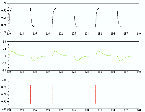
Figure 8.14: Scope window obtained with the values 0; -5; 0; 0; -5 for gains of the C₁ controller and 4; 4; -4; -4 for the C₂ controller.

8.6 SynDEx simulation

8.6.1 In the case of a mono-processor architecture

The architecture

In this subsection, we suppose that the architecture is constituted of an only operator named root:

create the U operator:

set the durations with

      
	float/delay = 1
	gain_def = 1
	scope_def = 1
	senseur_def = 2
	sommateur2_def = 2
	sommateur4_def = 1
	sommateur5_def = 2
	vitesse_def = 1

choose init as code generation phase in which to generate code;

create the mono architecture:
- add one U operator named root and define it as main operator,
- define the mono architecture as main.

The adequation and the code generation

First, launch the adequation. It modifies example8.sdc and example8.sdx files.

Then, generate the executive and applicative files (setting Code / Generate m4x Files). It creates example8.m4, example8.m4x, example8_sdc.m4x, and root.m4 files.

Finally, handwrite the example8.m4x file as explained in 8.4.6.

The compilation

First, generate manually a GNUmakefile containing:

  
    A  = example8
    M4 = gm4

    export ArchiMacros_Path = ../../../macros/archi_libraries
    export AlgoMacros_Path = ../../../macros/algo_libraries
    export M4PATH = $(ArchiMacros_Path):$(AlgoMacros_Path)

    CFLAGS = -DDEBUG
    VPATH = $(M4PATH)

    .PHONY: all clean
    all : $(A).mk $(A).run
    clean ::
    $(RM) $(A).mk *~ *.o *.a *.c actuator_*

    $(A).mk : $(A).m4 syndex.m4m U.m4m
    $(M4) $< >$@

    root.libs =
    P1.libs =

    include $(A).mk

Where:

A is set with the name of your application (here example8);
the path about the generic *.m4? macro-files are stored in the exported shell variables ArchiMacros_Path and AlgoMacros_Path then grouped into a new exported shell variable named M4PATH. The separator : means that a m4 macro-file will be search first in ArchiMacros_Path and then in AlgoMacros_Path if is not found;
a mix of this makefile and the informations stored in file named example8.m4m will create another makefile called example8.mk during the compilation.

Then, copy-paste the ref_vitesse.txt file from the Example 8 folder to yours.

Then, type the command gmake in a shell commands interpreter. It creates actuator_1, actuator_2, example8.mk, root, root.c, and root.root.o files:

the actuator_1 file contains the speed of the first car;
the actuator_2 file contains the distance between the cars.

8.6.2 In the case of a bi-processor architecture

The architecture

In this subsection, we suppose that the architecture is constituted of two operators named root and pc1, of type U and linked with a medium tcp1 of type TCP:

create the TCP medium:
- set the type with SAM MultiPoint,
- set the durations with float = 1;
modify the U operator: set the gates with TCP x and TCP y;
create the biProc architecture:
- add one U operator named root and define it as main operator,
- add one U operator named pc1,
- add one TCP medium named tcp1 and choose the Broadcast option,
- links the medium to the x gates of the operators,
- define the biProc architecture as main.

The adequation and the code generation

First, launch the adequation. It modifies example8.sdc and example8.sdx files.

Then, generate the executive and applicative files (setting Code / Generate m4x Files). It creates example8.m4, example8.m4x, example8_sdc.m4x, root.m4, and pc1.m4 files.

Finally, handwrite the example8.m4x file as explained in 8.4.6.

The compilation

First, generate manually the GNUmakefile, the example8.m4m, and the root.m4x files:

the GNUmakefile has to be created as explained in 8.6.1. Upgrade it so that the line:

    
      $(A).mk : $(A).m4 syndex.m4m U.m4m

is changed by:

    
      $(A).mk : $(A).m4 syndex.m4m U.m4m $(A).m4m

create the example8.m4m file with this line: define(‘pc1_hostname_’, HOSTNAME)dnl where HOSTNAME is substituted with the name of your remote station;
create the root.m4x file with this line: include(example8.m4m).

Then, copy-paste the ref_vitesse.txt file from the Example 8 folder to yours.

Then, type the command gmake in a shell commands interpreter. It creates actuator_1, actuator_2, example8.mk, root, root.c, root.root.o, pc1, pc1.c, and pc1.pc1.o files:

the actuator_1 file contains the speed of the first car;
the actuator_2 file contains the distance between the cars.

8.6.3 In the case of a multi-processor architecture

The architecture

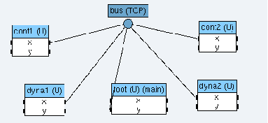
Figure 8.15: The architecture with 5 operators.

In this subsection, we suppose that the architecture is constituted of five operators named root,cont1, cont2, dyna1, and dyna2, of type U and linked with a medium bus of type TCP:

create the multi architecture (cf. figure 8.15):
- add one U operator named root and define it as main operator,
- add one U operator named cont1,
- add one U operator named cont2,
- add one U operator named dyna1,
- add one U operator named dyna2,
- add one TCP medium named bus and choose the Broadcast option,
- links the medium to the x gates of the operators, except for the root one, linked with its y gate to the medium,
- define the multi architecture as main;
create operation groups:
- create the og_root operation group, attach ref_vit, vitesse, and distance to it,
- create the og_dyna1 operation group, from the main mode, in the vehicule1 reference attach meca1 to it,
- create the og_cont1 operation group, from the main mode, in the vehicule1 reference attach control1 to it,
- create the og_dyna2 operation group, from the main mode in the vehicule2 reference attach meca2 to it,
- create the og_cont2 operation group, from the main mode, in the vehicule2 reference attach control2 to it;
create absolute constraints:
- constrain og_root on root,
- constrain og_cont1 on cont1,
- constrain og_cont2 on cont2,
- constrain og_dyna1 on dyna1,
- constrain og_dyna2 on dyna2.

The adequation and the code generation

First, launch the adequation. It modifies example8.sdc and example8.sdx files.

Then, generate the executive and applicative files (setting Code / Generate m4x Files). It creates example8.m4, example8.m4x, example8_sdc.m4x, root.m4, cont1.m4, cont2.m4, dyna1.m4, and dyna2.m4 files.

Finally, handwrite the example8.m4x file as explained in 8.4.6.

The compilation

First, generate manually the Makefile.ocaml, the example8.m4m, the root.m4x, the cont1.m4x, the cont2.m4x, the dyna1.m4x, and the dyna2.m4x files:

copy-paste the Makefile.ocaml from the Example 8 folder to yours;

create the example8.m4m file with these lines:

    
      define(‘cont1_hostname_’, HOSTNAME)dnl
      define(‘cont2_hostname_’, HOSTNAME)dnl
      define(‘dyna1_hostname_’, HOSTNAME)dnl
      define(‘dyna2_hostname_’, HOSTNAME)dnl

where HOSTNAME is substituted with the name of your remote station;

create the root.m4x, cont1.m4x, cont2.m4x, dyna1.m4x, and dyna2.m4x files with this line: include(example8.m4m).

Then, copy-paste some files from the Example 8 folder to yours:

copy-paste the example8.ml file.
copy-paste the pa_example8.ml file.
copy-paste the root.sh, cont1.sh, cont2.sh, dyna1.sh, and dyna2.sh files;
copy-paste the ref_vitesse.txt file.

You will probably need to install camlp5 (see at http://pauillac.inria.fr/ ddr/camlp5/).

Then, type the command make -f Makefile.ocaml in a shell commands interpreter. It creates example8.cmi, example8.o, pa_example8.cmi, and <processor>.cmi, <processor>.cmx, <processor>.o, <processor>.opt for each processor.

Finally, launch separatly the five script files. At the end of their execution, the actuator_1 and actuator_2 files are created:

the actuator_1 file contains the speed of the first car;
the actuator_2 file contains the distance between the cars.

From the principal window, choose File / Close. In the dialog window, click on the Save button.

1: http://www.scilab.org

Chapter 8 Example 8: a complete realistic application from adequation to execution

8.1 The aim of the example

8.2 The model

8.3 The controllers

8.3.1 Block diagrams of controllers

8.3.2 Source code associated with the functions

Gain

Sum

8.4 The complete model

8.4.1 The car dynamics

8.4.2 The cars and their controllers

8.4.3 The main algorithm

8.4.4 Source code associated with the sensor and the actuator

Input

Speed output

Distance output

8.4.5 The example8_sdc.m4x

8.4.6 To handwrite the example8.m4x file

8.5 Scicos simulation

8.6 SynDEx simulation

8.6.1 In the case of a mono-processor architecture

The architecture

The adequation and the code generation

The compilation

8.6.2 In the case of a bi-processor architecture

The architecture

The adequation and the code generation

The compilation

8.6.3 In the case of a multi-processor architecture

The architecture

The adequation and the code generation

The compilation

8.4.5 The `example8_sdc.m4x`

8.4.6 To handwrite the `example8.m4x` file